Tutorial: layout presets

One function, five templates. Pick a template, give the country → region steps, and (optionally) terrain=True for a relief focus panel. Sizes and connectors are fully customizable.

This tutorial uses India → Uttarakhand → Chamoli. The terrain panels need pip install "acadgis[terrain]".

Setup

import acadgis as agis
print("AcadGIS", agis.__version__)
print("templates:", list(agis.TEMPLATES))

STATE, DISTRICT = "Uttarakhand", "Chamoli"
S1    = [("district", DISTRICT)]                       # focus only
S_two = [("state", STATE)]                             # country + state
S2    = [("state", STATE), ("district", DISTRICT)]     # country -> state -> district

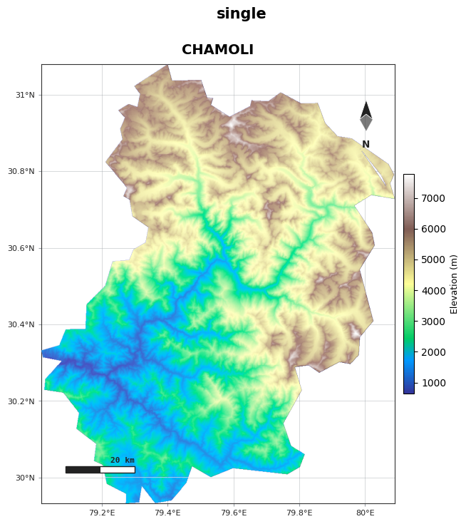
1. single — one map

agis.study_area("India", steps=S1, template="single", terrain=True, suptitle="single")

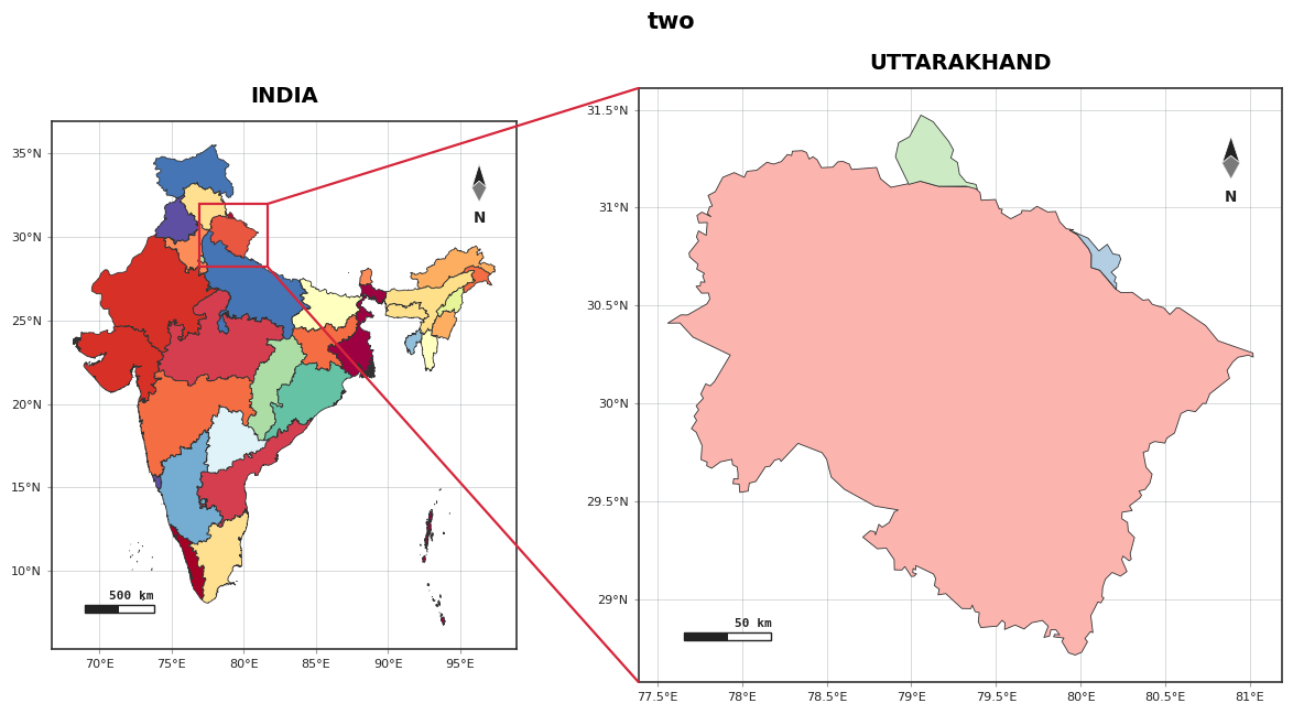
2. two — smaller context + larger focus

agis.study_area("India", steps=S_two, template="two", suptitle="two")

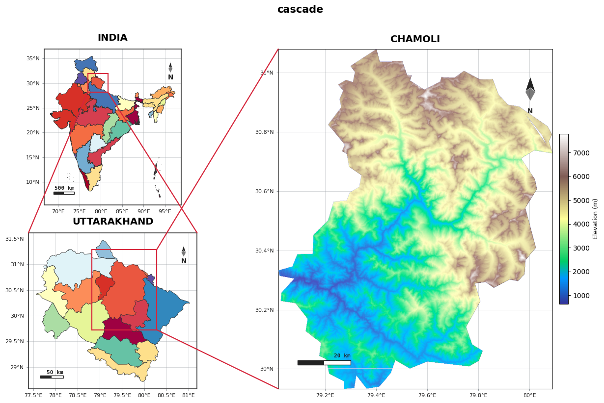
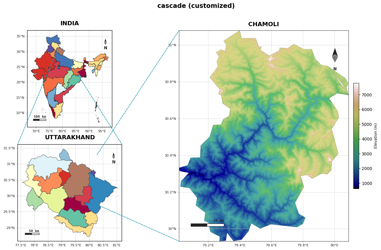
3. cascade — two small panels + one big focus (terrain last)

agis.study_area("India", steps=S2, template="cascade", terrain=True, suptitle="cascade")

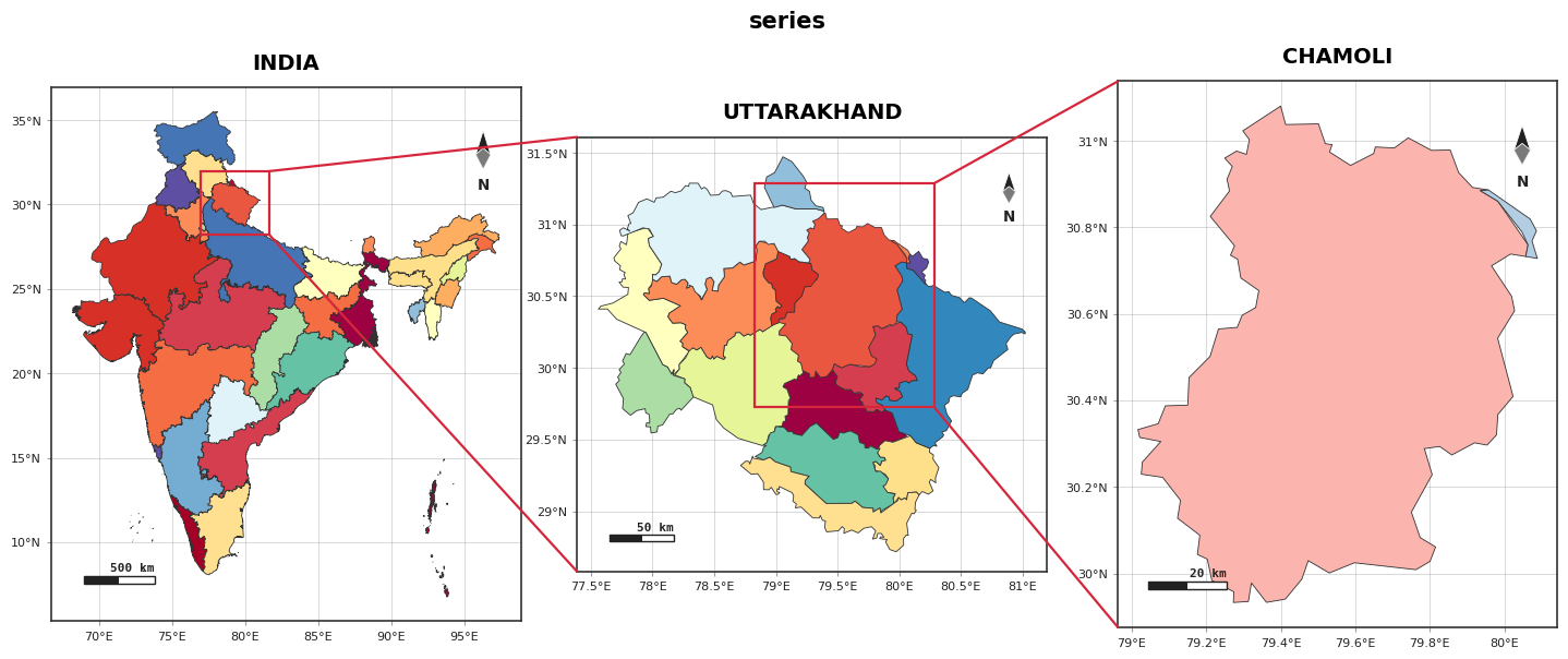
4. series — three uniform panels in a row

agis.study_area("India", steps=S2, template="series", suptitle="series")

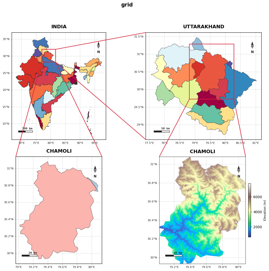
5. grid — 2 × 2 uniform

agis.study_area("India", steps=S2, template="grid", terrain=True, suptitle="grid")

6. Customized cascade

Everything is overridable — width_ratios, height_ratios, wspace, hspace, link_color, link_width, link_style, box, highlight_color, palette, cmap, figsize:

agis.study_area("India", steps=S2, template="cascade", terrain=True,
                width_ratios=[1, 2.2], link_color="#1b9aaa",
                link_style="--", link_width=1.2, box=False,
                highlight_color="#1b9aaa", cmap="gist_earth",
                suptitle="cascade (customized)")

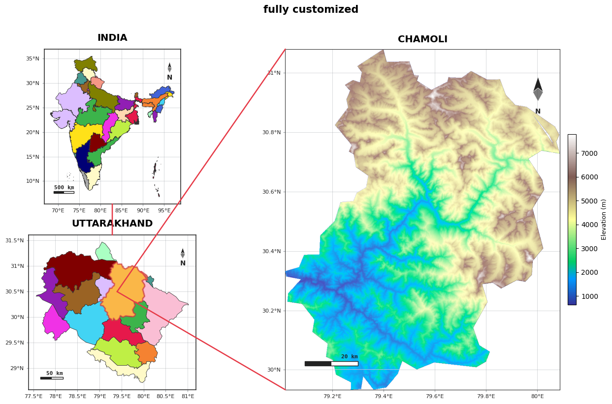
7. All customizations together

Every study_area knob — panel sizes, colours and connectors — plus a manual highlight and hand-placed connectors using fig.panels + ConnectionPatch. Coordinate systems: transData = map lon/lat, transAxes = panel 0–1, transFigure = whole figure.

from matplotlib.patches import ConnectionPatch

fig = agis.study_area(
    "India", steps=S2, template="cascade", terrain=True,
    # panel sizes
    width_ratios=[1, 2.0], height_ratios=[1, 1], wspace=0.10, hspace=0.20,
    figsize=(16, 9),
    # colours
    palette="vibrant", detail_palette="earth", cmap="terrain",
    highlight_color="#e63946", highlight_alpha=0.40,
    # built-in connectors off — we hand-draw below
    links=False, box=True,
    suptitle="fully customized",
)

axA, axB, axC = fig.panels[:3]

# custom highlight overlay on the state panel
uk = agis.load_boundaries("India", "district", within=STATE)
chamoli = uk[uk["NAME_2"] == DISTRICT]
chamoli.plot(ax=axB, facecolor="#ffd166", alpha=0.5, edgecolor="#e63946",
             linewidth=2.5, zorder=9)

# India (bottom-middle) -> Uttarakhand (top-middle)
fig.add_artist(ConnectionPatch(xyA=(0.5, 0.0), coordsA=axA.transAxes,
                               xyB=(0.5, 1.0), coordsB=axB.transAxes,
                               color="#e63946", lw=1.8, zorder=50, clip_on=False))
# a fixed map point on Uttarakhand -> both left corners of the Chamoli panel
for corner in [(0.0, 1.0), (0.0, 0.0)]:
    fig.add_artist(ConnectionPatch(xyA=(79.4, 30.5), coordsA=axB.transData,
                                   xyB=corner, coordsB=axC.transAxes,
                                   color="#e63946", lw=1.8, zorder=50, clip_on=False))

agis.plt.show()

Notes

• single = 1 panel, two = 2, cascade/series = 3, grid = 4.
• terrain=True makes the largest/last panel shaded relief (Copernicus GLO-30, cached).
• Save any figure: fig = agis.study_area(...) then agis.save(fig, "study.png", dpi=300).

See the Study-area layouts guide for every parameter.