Tutorial: India → West Bengal → Kolkata

A study-area figure that ends with collected data — synthetic sampling sites around Kolkata, drawn as graduated symbols. Runs on the bundled India data.

1. Set up

import acadgis as agis

STEPS = [("state", "West Bengal"), ("district", "Kolkata")]

2. The locator figure

agis.study_area("India", steps=STEPS, template="cascade",
                suptitle="Study area: Kolkata, West Bengal")

3. Make some synthetic sampling data

import numpy as np
rng = np.random.default_rng(42)

n = 40
survey = agis.pd.DataFrame({
    "name":  [f"S{i:02d}" for i in range(n)],
    "lon":   88.30 + rng.normal(0, 0.06, n),
    "lat":   22.57 + rng.normal(0, 0.06, n),
    "value": rng.gamma(2.0, 12.0, n).round(1),
})

4. Plot the district with graduated symbols

Draw the Kolkata polygon, then overlay the sites coloured and sized by value:

kolkata = agis.load_boundaries("India", "district", within="West Bengal")
kolkata = kolkata[kolkata["NAME_2"] == "Kolkata"]

ax = agis.plot(kolkata, palette="pastel", title="Kolkata — sampling sites")
agis.points(ax, survey, value="value", size_by="value",
            cmap="magma", legend=True, label="name")
agis.show()

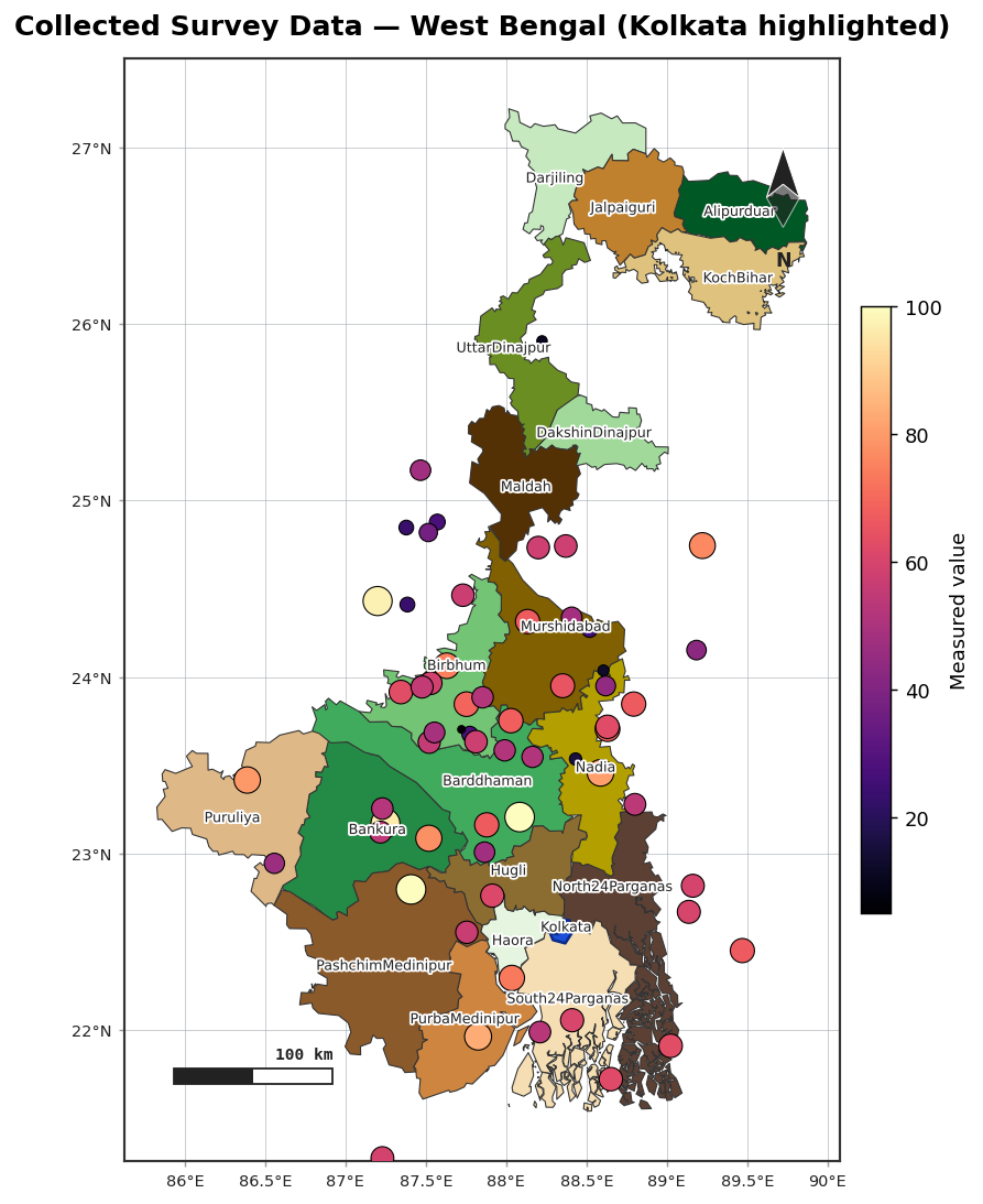
5. Or layer points over a choropleth

If you have district-level values too, combine both encodings:

ax = agis.choropleth(
    agis.load_boundaries("India", "district", within="West Bengal"),
    district_df, value="cases", palette="viridis", scheme="quantiles",
)
agis.points(ax, survey, value="value", size_by="value", legend=True)
agis.save("kolkata_survey.png", dpi=300)

6. Export

agis.save("kolkata_study.pdf", dpi=300)

That's the full arc — boundaries, a locator layout, and collected data — in a handful of lines. Explore the User guide for every option, or the API reference.